« Previous « Start » Next »
48 Hang Glider Control
Benchmarking Optimization Software with COPS Elizabeth D. Dolan and Jorge J. More ARGONNE NATIONAL LABORATORY
48.1 Problem Formulation
Find u(t) over t in [0; t_F ] to maximize
subject to:
| = | | *(−L*sin(neta)−D*cos(neta)) |
| = | | *(L*cos(neta)−D*sin(neta)) − g |
| D = | | *(c0+c1**cL2)*rho*S*v2 |
cL is the control variable.
Reference: [14]
48.2 Problem setup
toms t
toms t_f

for n=[10 80]
    p = tomPhase('p', t, 0, t_f, n, [], 'cheb');
    setPhase(p);

    tomStates x dx y dy
    tomControls cL

    % Initial guess
    % Note: The guess for t_f must appear in the list before
    % expression involving t.
    if n == 10
        x0 = {t_f == 105
            icollocate({
            dx == 13.23; x  == dx*t
            dy == -1.288; y  == 1000+dy*t
            })
            collocate(cL==1.4)};
    else
        x0 = {t_f == tf_opt
            icollocate({
            dx == dx_opt; x  == x_opt
            dy == dy_opt; y  == y_opt
            })
            collocate(cL == cL_opt)};
    end

    % Box constraints
    cbox = {
        0.1 <= t_f <= 200
        0   <= icollocate(x)
        0   <= icollocate(dx)
        0   <= collocate(cL) <= 1.4};

    % Boundary constraints
    cbnd = {initial({x  == 0; dx == 13.23
        y  == 1000; dy == -1.288})
        final({dx == 13.23; y  == 900; dy == -1.288})};

    % Various constants and expressions
    m = 100;      g = 9.81;
    uc = 2.5;     r0 = 100;
    c0  = 0.034;  c1  = 0.069662;
    S   = 14;     rho = 1.13;

    r = (x/r0-2.5).^2;
    u = uc*(1-r).*exp(-r);
    w = dy-u;
    v = sqrt(dx.^2+w.^2);
    sinneta = w./v;
    cosneta = dx./v;
    D = 1/2*(c0+c1*cL.^2).*rho.*S.*v.^2;
    L = 1/2*cL.*rho.*S.*v.^2;

    % ODEs and path constraints
    ceq = collocate({
        dot(x)  == dx
        dot(dx) == 1/m*(-L.*sinneta-D.*cosneta)
        dot(y)  == dy
        dot(dy) == 1/m*(L.*cosneta-D.*sinneta)-g
        dx.^2+w.^2 >= 0.01});

    % Objective
    objective = -final(x);
48.3 Solve the problem
    options = struct;
    options.name = 'Hang Glider';
    solution = ezsolve(objective, {cbox, cbnd, ceq}, x0, options);
Problem type appears to be: lpcon
Starting numeric solver
===== * * * =================================================================== * * *
TOMLAB - Tomlab Optimization Inc. Development license  999001. Valid to 2011-02-05
=====================================================================================
Problem: ---  1: Hang Glider                    f_k   -1281.388593956430400000
                                       sum(|constr|)      0.000000000082304738
                              f(x_k) + sum(|constr|)  -1281.388593956348100000
                                              f(x_0)  -1389.149999999999600000

Solver: snopt.  EXIT=0.  INFORM=1.
SNOPT 7.2-5 NLP code
Optimality conditions satisfied

FuncEv    1 ConstrEv   55 ConJacEv   55 Iter   37 MinorIter  191
CPU time: 0.250000 sec. Elapsed time: 0.250000 sec.
Problem type appears to be: lpcon
Starting numeric solver
===== * * * =================================================================== * * *
TOMLAB - Tomlab Optimization Inc. Development license  999001. Valid to 2011-02-05
=====================================================================================
Problem: ---  1: Hang Glider                    f_k   -1305.253702077266800000
                                       sum(|constr|)      0.000000045646790482
                              f(x_k) + sum(|constr|)  -1305.253702031619900000
                                              f(x_0)  -1281.388593956420700000

Solver: snopt.  EXIT=0.  INFORM=1.
SNOPT 7.2-5 NLP code
Optimality conditions satisfied

FuncEv    1 ConstrEv   80 ConJacEv   80 Iter   67 MinorIter  801
CPU time: 4.468750 sec. Elapsed time: 4.547000 sec.
48.4 Extract optimal states and controls from solution
    x_opt  = subs(x,solution);
    dx_opt = subs(dx,solution);
    y_opt  = subs(y,solution);
    dy_opt = subs(dy,solution);
    cL_opt = subs(cL,solution);
    tf_opt = subs(t_f,solution);
end
48.5 Plot result
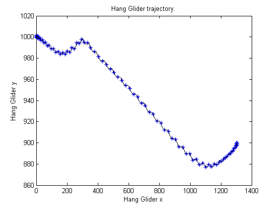
figure(1)
ezplot(x,y);
xlabel('Hang Glider x');
ylabel('Hang Glider y');
title('Hang Glider trajectory.');
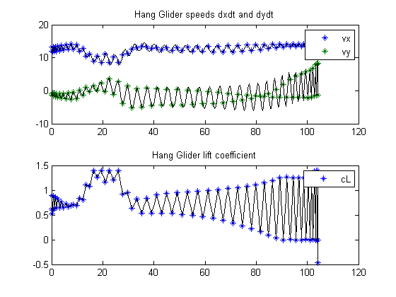
figure(2)
subplot(2,1,1)
ezplot([dx; dy]);
legend('vx','vy');
title('Hang Glider speeds dxdt and dydt');
subplot(2,1,2)
ezplot(cL);
legend('cL');
title('Hang Glider lift coefficient');
« Previous « Start » Next »